Functions for Formulas
Last updated on 2025-10-30
Overview
In the following tables you will find functions that you can use in xP&A formulas.
This article contains the following sections:
Available Formulas
The following functions are available for formulas in Lucanet xP&A:
Math
Function
Description
abs
The absolute value of a number
avg
The arithmetic mean (average) of the inputs. Can also be used as avgif.
Example: avg(1, 2, 3) = 2avg(if Var[all] % 2 = 0 then Var[all] else none = avg of all even values
first_nonzero_value
The first value that is not zero or empty
Example: first_nonzero_value(0,none,4,6) = 4
log
Natural logarithm (base e)
Example: log(e^2) = 2
log10
Common logarithm (base 10)
Example: log10(100) = 2
max
The highest of the given values
Example: max(1, 2, 3) = 3; max([1, 2, 3]) = 3
min
The lowest of the given values
Example: min(1, 2, 3) = 1; min([1, 2, 3]) = 1
mod
The remainder of a division.You can also use mod as "%"
Example: mod(5, 2) = 15 % 2 = 1reccurence every 4 months: if timeStep % 4 = 0 then 1 else 0
reverse
Reverses the order of an array.
Example: reverse([1, 2]) = [2, 1]
round
Rounds the number to the closest integer. Optionally, you can specify the decimal places as the second argument.
Example: round(2.3) = 2, round(2.5) = 3, round(2.26, 1) = 2.3
rounddown
Rounds the number down, toward 0. Optionally, you can specify the decimal places as the second argument.
Example: rounddown(2.8) = 2, rounddown(-2.8) = -2, rounddown(2.88, 1) = 2.8
roundup
Rounds the number up, away from 0. Optionally, you can specify the decimal places as the second argument.
Example: roundup(2.2) = 3, roundup(-2.2) = -3, roundup(2.22, 1) = 2.3
signchange
Timestep on which the first sign change occurs
Example: signchange(Var[all])
spread
Spreads a value over a time period.
Example: spread(New Customers[0:t], Payments[0:t])
For a more detailed example, see Examples for Functions.
sqrt
Square root of a value
Example: sqrt(4) = 2
sum
The sum of the inputs. Can also be used as sumif or countif.
Example: sum(1, 2, 3) = 6. sum(if Var[all] % 2 = 0 then Var[all] else 0) = sum of all even values
sumproduct
Multiplies two or more arrays together and returns the sum of products.
Example: sumproduct(Var1[all], Var2[all])
exp
Exponential function
Example: exp(2) = e^2
Time
Function
Description
date
The timestep number of a date. Timesteps start with 0.
Example: date(2021,12,24) = 11 in a monthly model that starts in Jan 2021
month_from_date
Extracts the month of a date or timestep.
Example: month_from_date( date(2021,12,24) ) = 12
year_from_date
Extracts the year of a date or timestep.
Example: year_from_date( date(2021,12,24) ) = 2021
Financial
Function
Description
cumipmt
Cumulative interest paid.
Example: cumipmt(rate, periods, value, start, end, type)
finance.AM
Amortization
Example: finance.AM(principal, rate, period, yearOrMonth, payAtBeginning)
finance.CAGR
Compound annual growth rate
Example: finance.CAGR(beginning value, ending value, number of periods)
finance.CI
Compound interest
Example: finance.CI(rate, compoundings per period, principal, number of periods)
finance.DF
Discount factor (returns an array; must index array to obtain values -- to see all values of array, see working example above).
Example: finance.DF(rate, number of periods)[index]
finance.FV
Future value
Example: finance.FV(rate, nper, pmt, pv, type)
finance.IAR
Inflation-adjusted return
Example: finance.IAR(investment return, inflation rate)
finance.irr
Internal rate of return.
Example: finance.IRR(Cashflows[all], [guess])
For a more detailed example, see Examples for Functions.
finance.LR
Leverage ratio
Example: finance.LR(total liabilities, total debts, total income)
finance.NPV
Net present value
Example: finance.NPV(rate, initial investment, cash flows[all])
For a more detailed example, see Examples for Functions.
finance.PI
Profitability index
Example: finance.PI(rate, initial investment, cash flows[all])
finance.PMT
Payment for a loan based on constant payments and a constant interest rate
Example: finance.PMT(fractional interest rate, number of payments, principal)
finance.PP
Payback period
Example: finance.PP(number of periods, cash flows[all])
finance.PV
Present value
Example: finance.PV(rate, nper, pmt, [fv], [type])
finance.R72
Rule of 72
Example: finance.R72(rate)
finance.roi
Return on investment
Example: finance.ROI(Cashflows[all])
finance.WACC
Weighted average cost of capital
Example: finance.WACC(market value of equity, market value of debt, cost of equity, cost of debt, tax rate)
finance.xirr
Internal rate of return for a schedule of cash flows
Example: finance.xirr([-10,11], [0,12], 12) = 10%
For a more detailed example, see Examples for Functions.
fv
Future value
Example: v(rate, nper, pmt, pv, [type])
fvifa
Future value interest factor of an annuity
Example: fvifa(rate, nper)
ipmt
Interest portion of a given loan payment
Example: ipmt(rate, per, nper, pv, [fv], [type])
pmt
Periodic payment for a loan
Example: pmt(rate, nper, pv, [fv], [type])
ppmt
Principal portion of a given loan payment
Example: ppmt(rate, per, nper, pv, [fv], [type])
pv
Present value
Example: pv(rate, nper, pmt, fv, [type])
pvif
Present value interest factor
Example: pvif(rate, nper)
rate
Interest rate per period of an annuity
Example: rate(nper, pmt, pv, [fv], [type], [guess])
Probability
Function
Description
beta
Beta distribution
Example: beta(alpha, beta)
binominal
Binomial distribution
Example: binomial(n, p)
cauchy
Cauchy distribution
Example: cauchy(local, scale)
chisq
Chi-squared distribution
Example: chisq(k)
exponential
Exponential distribution
Example: exponential(rate)
gamma
Gamma distribution
Example: gamma(shape, scale)
invgamma
Inverse-gamma distribution
Example: invgamma(shape, scale)
lognormal
Log-normal distribution
Example: lognormal(μ, σ^2)
lognormal_from
Log-normal distribution
Example: finance.LR(total liabilities, total debts, total income)
normal
Net Present Value
Example: finance.NPV(rate, initial investment, cash flows[all])
normal_from
Log-normal distribution
Example: lognormal_from_interval (from, to, confidence_percent)
pareto
Pareto distribution
Example: pareto(min, alpha)
poisson
Poisson distribution
Example: poisson(λ)
stdev
The standard deviation of an array
Example: stdev(Var[all])
triangle
Triangle distribution
Example: triangle(from, to, confidence_percent)
uniform
Uniform distribution
Example: uniform(from, to)
variance
The variance of an array
Example: variance(Var[all])
Other
Function
Description
error
Error to assert an invalid state
Example: error()
flat_cohort_forecast
Forecasts cohort data without the cohort dimension.
Example: flat_cohort_forecast(oldCohorts[all], newCohorts[all], retentionRates[all], lastDataDate, t, [additionalChurn])
forecats
Forecasts your future inputs based on historical data using AI.
Example: forecast(timestep, past_values, growth_rate), where timestep is t and past_values references the variable with values.
Notes:
- Make sure you select a time period that has at least 13 inputs for the most accurate results, e.g. 13 months of data.
- growth_rate is optional.
gaussian_ramp
Ramps up a value over a time period in the shape of a gaussian bell curve.
Example: gaussian_ramp(timestep,date(2022,10), 2, 100)
if_error
If the first argument evaluates to an invalid number error, we return the second argument. Otherwise, we return the first argument.
Example: if_error(Y/X, Z) - useful where the denominator X is 0, and so the first argument would result in a divided by 0 (invalid number error)
is_data
Evaluates to 1 if argument is derived from a datasource, and otherwise to 0.
Example: is_data(Variable[all])
is_locked
Evaluates to 1 if argument is a locked dimension item, and otherwise to 0.
Example: is_locked(dimensionitem)
last_data_timestep
Returns the last timestep that is derived from a datasource.
Example:last_data_timestep(Var[all])
logistic_ramp
Ramps up a value over a time period in an S-shape (logistic function).
Example: logistic_ramp(timestep, date(2022,1), date(2022,10), 1.8, 100, 200)
quadratic_ramp
Ramps up a value quadratically over a time period.
Example: quadratic_ramp(timestep,date(2022,1), date(2022,10) [startValue], [endValue])
ramp
Ramps up a value linearly over a time period.
Example: ramp(timestep, date(2022,1), date(2022,10), 100, 200)
ramp_normalized
A ramp with the cumulative sum of 1. Useful for distributing a fixed value over a time period.
Example: ramp_normalized(timestep, date(2022,1), date(2022,10)
Examples for Functions
Use Case
Description
Spread values
Spread is a powerful and flexible xP&A function. It allows you to spread a value, or a set of values, over a time period. You can think of it as similar in functionality to sumproduct in Excel, but more intuitive (and of course, more powerful).
Spread has two arguments:
- x - the value or set of values
- y - the amount you are spreading x by
Example:
If all new customers have to pay a $100 sign-up fee in their first month, and from the second month onwards they pay $10 per month for their subscription - you could calculate your monthly revenue using spread.
In this instance, your x would be your new customers each month, and the y amount you are spreading it by would be that payment structure.
In xP&A, this would look as follows:
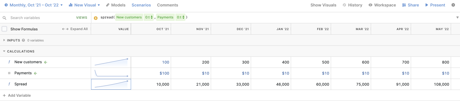 Example for 'spread' function
Other common use cases of spread are:
- Sales cycles (where ‘x’ is leads generated, and ‘y’ is the % that close over time)
- Retention curves (where ‘x’ is new users, and ‘y’ is the % that retain over time).
Internal Rate of Return (IRR)
xP&A has lots of finance functions that you might know from Excel or Google Sheets - and they work very similar.
Example:
If you have a Cash Flows variable where the first value is the initial investment and the following values are the returns, you can calculate the IRR like this:
 Example for 'finance.irr' function
Internal rate of return for a schedule of cash flows (XIRR):
XIRR is used when the cash flows are not periodic. That's why XIRR needs three arguments:
- The cashflows
- The time steps at which they occur
- The granularity (how many time steps fit into one year).
Example:
If you invest $10 in the first month and have a return of $6 after 10 months and another $6 after 12 months, your formula would look like this:
Net Present Value (NPV)
Net Present Value (NPV) compares the money received in the future to an amount of money received today, while accounting for time and interest. The arguments of the function are:
- Rate in percent
- Cash flows
Example:
For a discount rate of 10%, an initial investment of 500 and cashflows of 200, 300 and 200 you can use the function like this: finance.npv(10, -500, 200, 300, 200).
Usually the cashflows are in a time series variable, in this case you can use the variable in the function: