Using the Data View
Last updated on 2026-04-13
Overview
In Lucanet Disclosure Management, the data view is used to review report values (including details like history, comments, and validation) that have been imported from a source system and adjust them when necessary.
Discrepancies can occur when report values are imported in cents and results are displayed in thousands, for example. In such cases, cent values (which are rounded to the nearest thousand) differ from the original values. The data view makes it possible to correct these deviations manually.
The Data view function is only available for programmed Excel files.
- An MS Excel file is classed as programmed if it has a Name column, at least one Values column, and at least one Programming column, and at least one cell is programmed into the Programming column.
- If the Programming column is empty, the MS Excel file is not classed as programmed.
This article contains the following sections:
Video: Using the Data View
In the following video, you can see how to use the data view and adjust values:
Opening the Data View
To open the data view, proceed as follows:
- In the Dashboard, click the document that you wish to check.
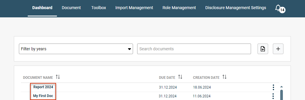 Opening a document from the Dashboard
 - To open the data view for a chapter, select one of the following options:
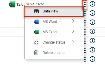
- Click the three dots icon
 of a chapter with a programmed MS Excel file and choose Data view:
Opening the data view from the cockpit - Click
 to open the detail view for a chapter and then click data view.
- Click the three dots icon
- The data view will display all the cells with report values from the MS Excel file associated with the chapter. The data view will be displayed as follows (for example):
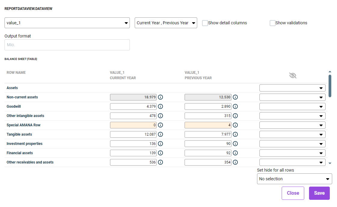 Data view in Disclosure Management
- The data view always displays all the rows programmed in the programming column of the MS Excel file in question.
- To display a value column in the data view with its column name from MS Excel, the cell that contains the column name must be configured accordingly (see Creating a Value Column).
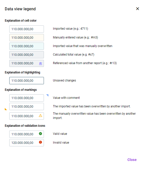
Colors and Symbols in the Data View
The cell colors and icons used in the data view indicate the type of values in a given report. The basic value types are:
- Automatic values: values imported from the source system
- Manually entered values: values entered manually by the user
Explanations of the colors and icons used can be opened by clicking the Legend button: